Overview
slendr is an R package toolbox for defining population genetic models and simulating genomic data entirely from R. It has been originally conceived as a framework for simulating spatially-explicit genomic data on real geographic landscapes but it has grown to be much more than that.
This page briefly summarizes slendr’s most important features. A a much detailed description of the slendr architecture and an extensive set of practical code examples can be found in our paper in the PCI journal and on our website.
Citing slendr
The slendr paper is now published in the Peer Community Journal!
If you use slendr in your work, please cite it as:
Petr, Martin; Haller, Benjamin C.; Ralph, Peter L.; Racimo, Fernando. slendr: a framework for spatio-temporal population genomic simulations on geographic landscapes. Peer Community Journal, Volume 3 (2023), article no. e121. doi : 10.24072/pcjournal.354.
Citations help me justify further development and fixing bugs! Thank you! ❤️
Main features
Here is a brief summary of slendr’s most important features. The R package allows you to:
Program demographic models, including population splits, population size changes, and gene-flow events using an extremely simple declarative language entirely in R (see this vignette for an example of the model-definition interface). Even complex models can be written with only a very little code and require only a bare minimum of R programming knowledge (the only thing the user needs to know is how to call an R function and what does an R data frame look like).
Execute slendr models using efficient, tailor-made SLiM or msprime simulation scripts which are bundled with the R package. Both of these simulation engines save outputs in the form of an efficient tree-sequence data structure. No SLiM or msprime programming is needed!
Load, process, and analyse tree-sequence outputs via slendr’s built-in R interface to the tree-sequence library tskit. You can compute many population genetic statistics in R immediately after the simulation finishes directly on the output tree sequences, without having to convert files to other formats (VCF, EIGENSTRAT) for analysis in different software.
Encode complex models of population movements on a landscape (see a brief example of such model here, and a more extended explanation in this tutorial). No knowledge of cartographic or geospatial analysis concepts is needed.
Simulate these dynamic spatial demographic models using SLiM’s continuous-space simulation capabilities directly in R (again, no SLiM programming required). The outputs from such simulations are saved as tree sequences and can be analysed using standard R geospatial data analysis libraries. This is because slendr performs the conversion of tree sequence tables to the appropriate spatial R data type automatically.
Specify within-population individual dispersal dynamics from the R interface by leveraging SLiM’s individual interaction parameters implemented in the SLiM back-end script.
Schedule sampling events which specify how many individuals’ genomes, from which populations, and at which times (optionally, at which locations) should be recorded by the simulation engine (SLiM or msprime) in the output tree-sequence files.
Utilizing the flexibility of R with its wealth of libraries for statistics, geospatial analysis and graphics, and combining it with the power of population genetic simulation frameworks SLiM and msprime, the slendr R package makes it possible to write entire simulation and analytic pipelines without the need to leave the R environment.
Testing the R package in an online RStudio session
You can open an RStudio session and test examples from the vignettes directly in your web browser by clicking this button (no installation is needed!):
![]()
In case the RStudio instance appears to be starting very slowly, please be patient (Binder is a freely available service with limited computational resources provided by the community). If Binder crashes, try reloading the web page, which will restart the cloud session.
Once you get a browser-based RStudio session, you can navigate to the vignettes/ directory and test the examples on your own!
Installation
slendr is now available CRAN which means that you can install it simply by entering install.packages("slendr") into your R console.
If you would like to test the latest features of the software (perhaps because you need some bug fixes), you can install it with devtools::install_github("bodkan/slendr") (note that this requires the R package devtools).
⚠️⚠️⚠️
Note: the default slendr installation no longer has a hard dependency on geospatial R packages sf, stars, and rnaturalearth. If you indend to use slendr for spatial genomic simulations and data analysis, you have to run install.packages(c("sf", "stars", "rnaturalearth")) first.
We made this change to ease the installation burden for researchers who might only need slendr’s support for traditional, non-spatial simulations (which represent the majority of use-cases in population genetics in general). The geospatial R packages imply a non-negligible amount of software dependencies themselves, which has proven to be an unnecessary hurdle for many users who might not need them (at least not at first).
⚠️⚠️⚠️
This software is under active development!
If you would like to stay updated:
Click on the “Watch” button on the project’s GitHub website.
Follow me on social media where I will be posting progress updates (you can find links on my homepage).
From time to time, take a look at the changelog where I will post updates on new features, breaking changes, etc.
Example
Here is a very brief demonstration of the kind of spatial model which slendr has been originally designed to simulate data from. Please note that although this is a spatially-explicit population genetic model, slendr has an extensive support for traditional, non-spatial simulations as well. Furthermore, this example only shows how to specify and simulate a model in R. It doesn’t show how to analyse tree-sequence outputs and compute population genetic statistics from them (this important feature is demonstrated in this tutorial).
1. Setup the spatial context
Imagine that we wanted to simulate spatio-temporal genomic data from a toy model of the history of modern humans in West Eurasia after the Out of Africa migration.
First, we define the spatial context of the simulation. This will represent the “world” which will be occupied by populations in our model.
library(slendr)

# this sets up internal Python environment and needs to be ran only once!
# (do not put this in your R scripts, run this command in the R console
# after you (re-)install slendr)
setup_env()

# activate the internal Python environment needed for simulation and
# tree-sequence processing
init_env()

map <- world(
  xrange = c(-13, 70), # min-max longitude
  yrange = c(18, 65),  # min-max latitude
  crs = "EPSG:3035"    # coordinate reference system (CRS) for West Eurasia
)
We can visualize the defined world map using the function plot_map provided by the package.
plot_map(map)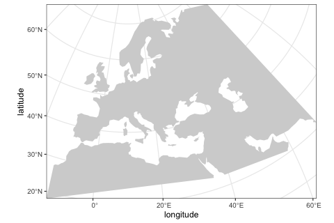
Although in this example we use a real Earth landscape, the map can be completely abstract (either blank or with user-defined landscape features such as continents, islands, corridors and barriers).
2. Define broader geographic regions
In order to make the definitions of population ranges (below) easier, we can define smaller regions on the map using the function region.
Note that all coordinates in slendr are specified in the geographic coordinate system (i.e., degrees longitude and latitude), but are internally represented in a projected CRS (in our case, EPSG 3035 as specified above).
This makes it easier for us to define spatial features simply by reading the coordinates from a regular map but the internal projected CRS makes simulations more accurate (distances and shapes are not distorted because we can use a CRS tailored to the region of the world we are working with). The projected CRS takes care of the projection of the part of the world we’re interested in from the three-dimensional Earth surface to a two-dimensional map.
africa <- region(
  "Africa", map,
  polygon = list(c(-18, 20), c(38, 20), c(30, 33),
                 c(20, 33), c(10, 38), c(-6, 35))
)
europe <- region(
  "Europe", map,
  polygon = list(
    c(-8, 35), c(-5, 36), c(10, 38), c(20, 35), c(25, 35),
    c(33, 45), c(20, 58), c(-5, 60), c(-15, 50)
  )
)
anatolia <- region(
  "Anatolia", map,
  polygon = list(c(28, 35), c(40, 35), c(42, 40),
                 c(30, 43), c(27, 40), c(25, 38))
)
Again, we can use the generic plot_map function to visualize these objects, making sure we specified them correctly:
plot_map(africa, europe, anatolia)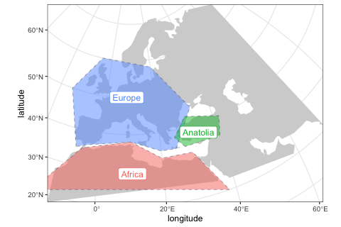
3. Define demographic history and population boundaries
The most important function in the slendr package is population(), which is used to define names, split times, sizes and spatial ranges of populations. Here, we specify times in years before the present, distances in kilometers. If this makes more sense for your models, times can also be given in a forward direction.
You will also note functions such as move() or expand_range() which are designed to take a slendr population object and schedule its spatial dynamics at appropriate times during the model simulation (which will happen at a later step).
Note that in order to make this example executable in a reasonable time on my extremely old laptop, I decreased the sizes of all populations to unrealistic levels. This will speed up the SLiM simulation at a later step.
afr <- population( # African ancestral population
  "AFR", time = 52000, N = 3000, map = map, polygon = africa
)

ooa <- population( # population of the first migrants out of Africa
  "OOA", parent = afr, time = 51000, N = 500, remove = 25000,
  center = c(33, 30), radius = 400e3
) %>%
  move(
    trajectory = list(c(40, 30), c(50, 30), c(60, 40)),
    start = 50000, end = 40000, snapshots = 20
  )

ehg <- population( # Eastern hunter-gatherers
  "EHG", parent = ooa, time = 28000, N = 1000, remove = 6000,
  polygon = list(
    c(26, 55), c(38, 53), c(48, 53), c(60, 53),
    c(60, 60), c(48, 63), c(38, 63), c(26, 60))
)

eur <- population( # European population
  name = "EUR", parent = ehg, time = 25000, N = 2000,
  polygon = europe
)

ana <- population( # Anatolian farmers
  name = "ANA", time = 28000, N = 3000, parent = ooa, remove = 4000,
  center = c(34, 38), radius = 500e3, polygon = anatolia
) %>%
  expand_range( # expand the range by 2.500 km
    by = 2500e3, start = 10000, end = 7000,
    polygon = join(europe, anatolia), snapshots = 20
  )

yam <- population( # Yamnaya steppe population
  name = "YAM", time = 7000, N = 500, parent = ehg, remove = 2500,
  polygon = list(c(26, 50), c(38, 49), c(48, 50),
                 c(48, 56), c(38, 59), c(26, 56))
) %>%
  move(trajectory = list(c(15, 50)), start = 5000, end = 3000, snapshots = 10)
We can use the function plot_map again to get a “compressed” overview of all spatio-temporal range dynamics encoded by the model so far (prior to the simulation itself).
plot_map(afr, ooa, ehg, eur, ana, yam)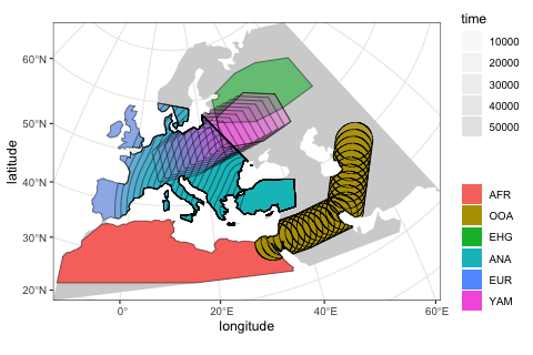
4. Define gene-flow events
By default, populations in slendr do not mix even if they are overlapping. In order to schedule an gene-flow event between two populations, we can use the function gene_flow. If we want to specify multiple such events at once, we can collect these events in a simple R list:
5. Compile the model to a set of configuration files
Before we run the simulation, we compile all individual model components (population objects and gene-flow events) to a single R object, specifying some additional model parameters. Additionally, this performs internal consistency checks, making sure the model parameters (split times, gene flow times, etc.) make sense before the (potentially quite computationally costly) simulation is even run.
model <- compile_model(
  populations = list(afr, ooa, ehg, eur, ana, yam), # populations defined above
  gene_flow = gf,
  generation_time = 30,
  resolution = 10e3,                   # resolution in meters per pixel
  competition = 130e3, mating = 100e3, # spatial interaction parameters
  dispersal = 70e3,                    # how far can offspring end up from their parents
)
Compiled model is kept as an R object which can be passed to different functions. In this example, we will simulate data with the slim() engine (but we could also run the simulation through the coalescent engine via the msprime() function).
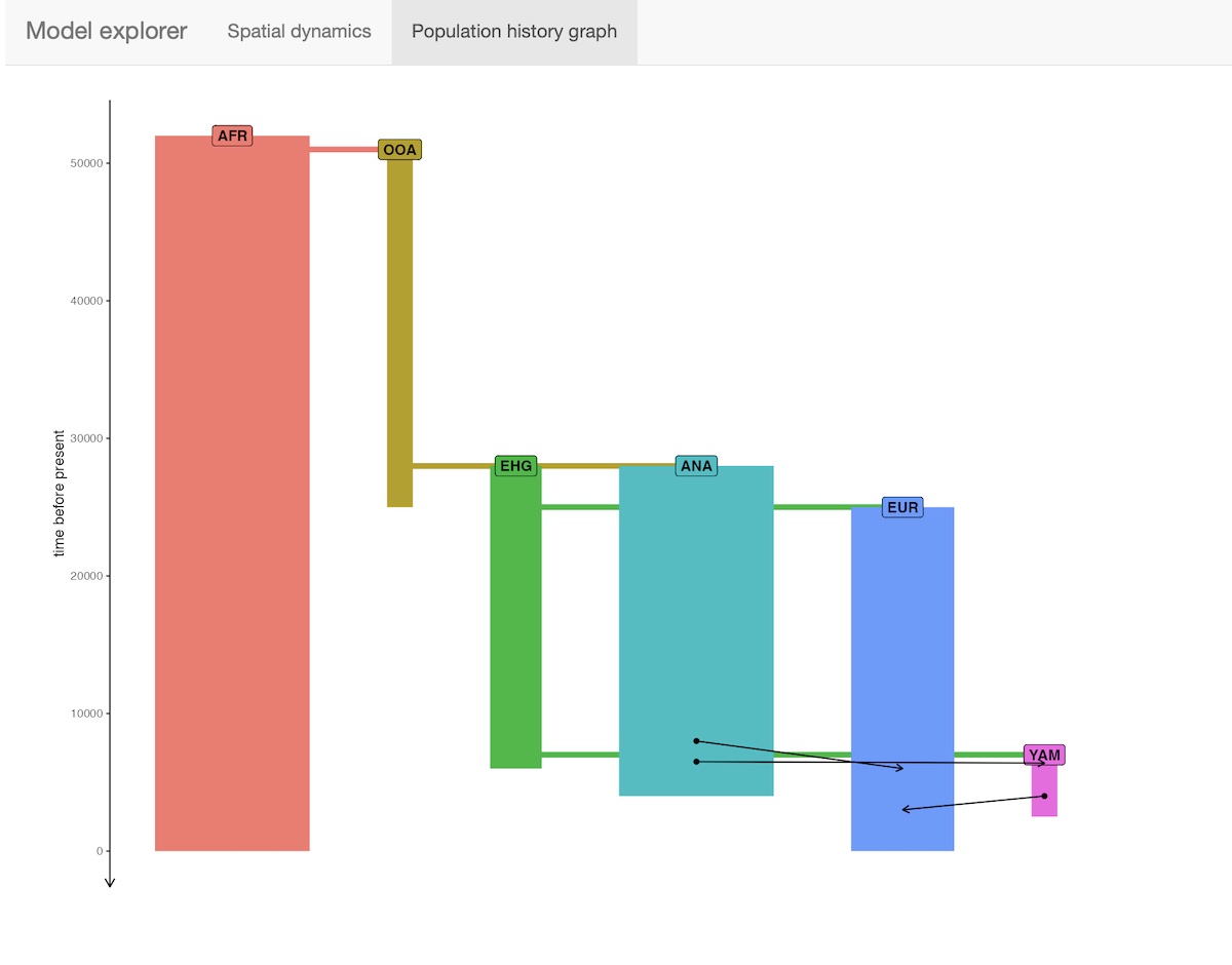
6. Visualize the model
The package provides an R shiny-based browser app explore_model() for checking the model dynamics interactively and visually. For more complex models, this is much better than static spatial plots such as the one we showed in step 2 above:
explore_model(model)The function has two modes:
- Plotting (and “playing”) spatial map dynamics:
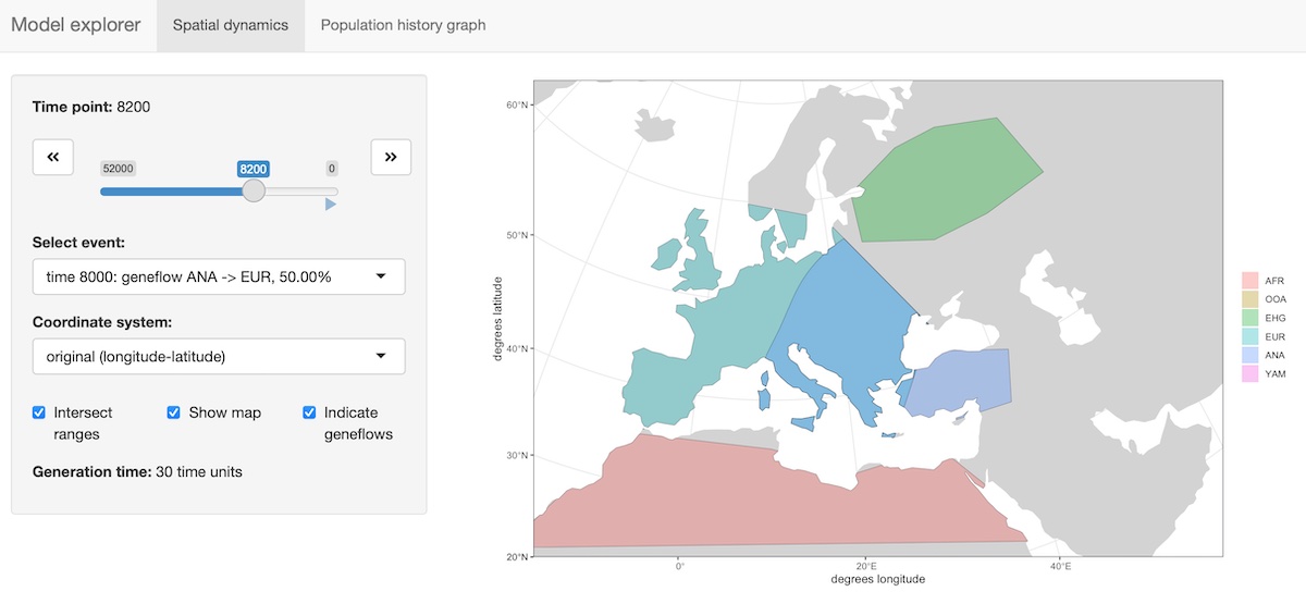
- Displaying the demographic history graph (splits and gene-flow events) embedded in the specified model:
7. Run the model in SLiM
Finally, we can execute the compiled model in SLiM. Here we run the simulation in a batch mode, but we could also run it in SLiMgui by setting method = "gui". This would allow us to inspect the spatial simulation as it happens in real time.
The slim function generates a complete SLiM script tailored to run the spatial model we defined above. This saves you, the user, a tremendous amount of time, because you don’t have to write new SLiM code every time you design a new demographic model. The output of the simulation run from any slendr model is always a tree sequence, here loaded into an object ts_slim.
ts_slim <- slim(model, sequence_length = 10e6, recombination_rate = 1e-8,
                method = "batch", random_seed = 314159)
As specified here, slendr’s SLiM backend will simulate 10 Mb of sequence for each individual, and produce a tree sequence output from the simulation run which can be analysed by many built-in population genetic functions. By default, all individuals living at the end of the simulation are recorded as samples in the tree sequence. If a specific set of samples (ancient and modern) is needed, this can be defined accordingly using a dedicated function.
Note that although we defined a spatial model, we could have just as easily simulated standard, non-spatial data by running the same model through slendr’s msprime() back end without the need to make any changes:
ts_msprime <- msprime(model, sequence_length = 10e6, recombination_rate = 1e-8)Here is a very quick overview of the SLiM simulation run summarised as a GIF animation. Again, please note that the simulation is extremely simplified. We only simulated a very small number of individuals in each population, and we also didn’t specify any dispersal dynamics which is why the populations look so clumped.
animate_model(model = model, file = locations_file, steps = 50, width = 500, height = 300)
At this point, you could either compute some population genetic statistics of interest or perhaps analyse the spatial features of the genealogies simulated by your model.
Further information
The example above provides only a very brief and incomplete overview of the full functionality of the slendr package. There is much more to slendr than what we demonstrated here. For instance:
You can tweak parameters influencing dispersal dynamics (how “clumpy” populations are, how far can offspring migrate from their parents, etc.) and define how these should change over time. For instance, you can see that in the animation above, the African population forms a single “blob” that really isn’t spread out across its entire population range. Tweaking the dispersal parameters as show this vignette helps avoid that.
You can use slendr to program non-spatial models, which means that any conceivable traditional, random-mating demographic model can be simulated with only a few lines of R code. You can learn more in this vignette (and in more detail in this vignette). Because SLiM simulations can be often quite slow compared to their coalescent counterparts, we also provide functionality allowing to simulate slendr models (without any change!) using a built-in msprime back end script. See this vignette for a tutorial on how this works.
You can build complex spatial models which are still abstract (not assuming any real geographic location), including traditional simulations of demes in a lattice structure. A complete example is shown this vignette.
Because slendr & SLiM save data in a tree-sequence file format, thanks to the R package reticulate for interfacing with Python code, we have the full power of tskit and pyslim for manipulating tree-sequence data right at our fingertips, all within the convenient environment of R. An extended example can be found in this vignette.
For spatially explicit population models, the slendr package automatically converts the simulated output data to a format which makes it possible to analyse it with many available R packages for geospatial data analysis. A brief description of this functionality can be found in this vignette.
You can find complete reproducible code behind the examples in our paper in a dedicated R vignette here.