Please note that the tspop support in
slendr implemented in the ts_tracts() function is
extremely experimental, only minimally tested, and its functionality is
expected to change quite a bit. Please wait for the release of the next
major version of slendr (which should include a more developed
ts_tracts()) before you use this in your own
work.
slendr now includes an experimental, use-it-at-your-own-risk interface to an exciting new algorithm for extracting true tracts of ancestry as implemented in the Python module tspop.
The interface is implemented in an R function
ts_tracts() and this vignette describes its use on a simple
toy model of Neanderthal and Denisovan introgression into modern
humans.
Demographic model
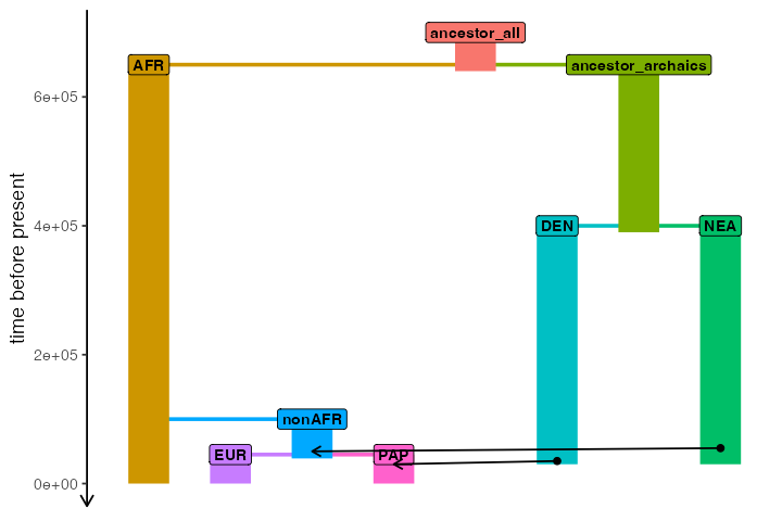
Let’s imagine the following demographic model of Neanderthal introgression into the ancestors of all non-Africans (represented by “EUR” and “PAP” populations, approximating European and Papuan people living today), followed by Denisovan introgression into the ancestors of Papuans:
anc_all <- population("ancestor_all", time = 700e3, N = 10000, remove = 640e3)
afr <- population("AFR", parent = anc_all, time = 650e3, N = 10000)
anc_arch <- population("ancestor_archaics", parent = anc_all, time = 650e3, N = 10000, remove = 390e3)
nea <- population("NEA", parent = anc_arch, time = 400e3, N = 2000, remove = 30e3)
den <- population("DEN", parent = anc_arch, time = 400e3, N = 2000, remove = 30e3)
nonafr <- population("nonAFR", parent = afr, time = 100e3, N = 3000, remove = 39e3)
eur <- population("EUR", parent = nonafr, time = 45e3, N = 5000)
pap <- population("PAP", parent = nonafr, time = 45e3, N = 5000)

gf <- list(
  gene_flow(from = nea, to = nonafr, rate = 0.03, start = 55000, end = 50000),
  gene_flow(from = den, to = pap, rate = 0.07, start = 35000, end = 30000)
)

model <- compile_model(
  populations = list(anc_all, afr, anc_arch, nea, den, nonafr, eur, pap),
  gene_flow = gf,
  generation_time = 30,
  serialize = FALSE
)

plot_model(
  model, sizes = FALSE,
  order = c("AFR", "EUR", "nonAFR", "PAP", "ancestor_all", "DEN", "ancestor_archaics", "NEA")
)
Tree sequence simulation
Let’s now simulate a 50Mb tree sequence from this model, recording 50 diploid individuals from EUR and PAP populations:
samples <- schedule_sampling(model, times = 0, list(eur, 50), list(pap, 50))

ts <- msprime(model, sequence_length = 100e6, recombination_rate = 1e-8, samples = samples, random_seed = 42)
Extracting ancestry tracts
In order to extract tracts of Neanderthal and Denisovan ancestry, we
can use slendr’s new function ts_tracts() which
serves as a simplified R-friendly interface to the Python method tspop.get_pop_ancestry().
An important piece of information used by the function is a so-called
“census time”, which records the time of recording of the “ancestral
population” identity of each node ancestral to each subsegment in our
sample set. Please see the excellent vignette of
tspop for more information on the inner workings of the
algorithm.
In our case, let’s extract the ancestry tracts corresponding to ancestral nodes present at 55 thousand years ago – this time corresponds to the moment of the start of the archaic introgression:
nea_tracts <- ts_tracts(ts, census = 55000)
#>
#> PopAncestry summary
#> Number of ancestral populations:     3
#> Number of sample chromosomes:        200
#> Number of ancestors:             44052
#> Total length of genomes:         20000000000.000000
#> Ancestral coverage:          20000000000.000000
den_tracts <- ts_tracts(ts, census = 35000)
#>
#> PopAncestry summary
#> Number of ancestral populations:     3
#> Number of sample chromosomes:        200
#> Number of ancestors:             55373
#> Total length of genomes:         20000000000.000000
#> Ancestral coverage:          20000000000.000000

tracts <- bind_rows(nea_tracts, den_tracts)
This is what a table with all ancestry tracts looks like. As we would expect, we see a column indicating a name of each individual, the left and right coordinates of each tract in each individual, as well as the population name of the source of each ancestry tract:
tracts
#> # A tibble: 17,002 × 8
#>    name  node_id pop   source_pop     left    right length source_pop_id
#>    <chr>   <dbl> <fct> <fct>         <dbl>    <dbl>  <dbl>         <dbl>
#>  1 EUR_1       0 EUR   NEA          781887   852668  70781             3
#>  2 EUR_1       0 EUR   NEA         1451389  1463837  12448             3
#>  3 EUR_1       0 EUR   NEA         1596995  1601441   4446             3
#>  4 EUR_1       0 EUR   NEA         1629857  1689656  59799             3
#>  5 EUR_1       0 EUR   NEA         3203711  3339565 135854             3
#>  6 EUR_1       0 EUR   NEA         3850629  3947923  97294             3
#>  7 EUR_1       0 EUR   NEA         6190700  6205627  14927             3
#>  8 EUR_1       0 EUR   NEA        10394211 10426667  32456             3
#>  9 EUR_1       0 EUR   NEA        13044685 13180258 135573             3
#> 10 EUR_1       0 EUR   NEA        14858956 14912068  53112             3
#> # ℹ 16,992 more rows
Summaries of ancestral proportions
When we summarise the ancestry proportions in target EUR and PAP populations, we see that the EUR population only carries about ~3% of Neanderthal ancestry and that this is also true for the PAP population. However, we also see that Papuans carry about 7% of Denisovan ancestry. This is consistent with our model, but also with the expectation from empirical data.
summary <- tracts %>%
  group_by(name, node_id, pop, source_pop) %>%
  summarise(prop = sum(length) / 100e6)
#> `summarise()` has grouped output by 'name', 'node_id', 'pop'. You can override
#> using the `.groups` argument.

summary %>% group_by(pop, source_pop) %>% summarise(mean(prop)) %>% arrange(source_pop, pop)
#> `summarise()` has grouped output by 'pop'. You can override using the `.groups`
#> argument.
#> # A tibble: 3 × 3
#> # Groups:   pop [2]
#>   pop   source_pop `mean(prop)`
#>   <fct> <fct>             <dbl>
#> 1 EUR   NEA              0.0303
#> 2 PAP   NEA              0.0348
#> 3 PAP   DEN              0.0739
Let’s visualize these proportions at an individual level:
summary %>%
ggplot(aes(source_pop, prop, color = source_pop, fill = source_pop)) +
  geom_jitter() +
  coord_cartesian(ylim = c(0, 0.2)) +
  geom_hline(yintercept = c(0.03, 0.08), linetype = 2) +
  ylab("ancestry proportion") +
  facet_wrap(~ pop) +
  ggtitle("Ancestry proportions in each individual",
          "(vertical lines represent 3% and 7% baseline expectations")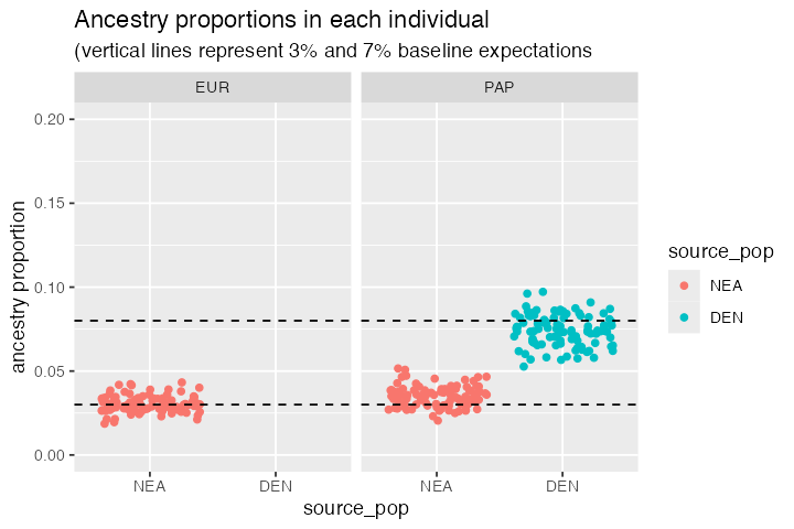
“Chromosome painting” of ancestry tracts
Because the tracts object contains the coordinates of
every single ancestry segment in each of the simulated individuals, we
can “paint” each chromosome with each of the two archaic human
ancestries:
tracts %>%
mutate(chrom = paste(name, " (node", node_id, ")")) %>%
ggplot(aes(x = left, xend = right, y = chrom, yend = chrom, color = source_pop)) +
  geom_segment(linewidth = 3) +
  theme_minimal() +
  labs(x = "position [bp]", y = "haplotype") +
  ggtitle("True ancestry tracts along each chromosome") +
  theme(axis.text.y = element_blank(), panel.grid = element_blank()) +
  facet_grid(pop ~ ., scales = "free_y")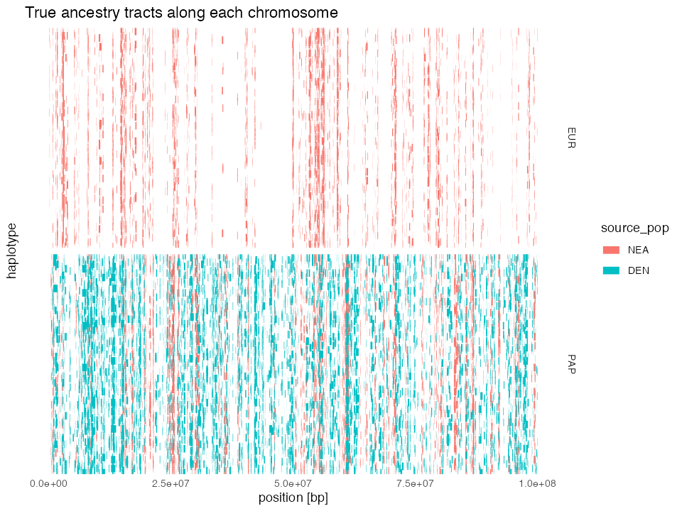
By lining up NEA & DEN ancestry tracts in both EUR and PAP populations, we can see how the common origin of Neanderthal ancestry in both non-African populations manifests in a significant overlap of NEA tracts between both populations.
Average tract lengths:
Let’s compute simple summaries of tract lengths in the simulated data, and compare them to theoretical expectations.
tracts %>%
  group_by(pop, source_pop) %>%
  summarise(mean(length))
#> `summarise()` has grouped output by 'pop'. You can override using the `.groups`
#> argument.
#> # A tibble: 3 × 3
#> # Groups:   pop [2]
#>   pop   source_pop `mean(length)`
#>   <fct> <fct>               <dbl>
#> 1 EUR   NEA                65765.
#> 2 PAP   NEA                69204.
#> 3 PAP   DEN               100317.
Theoretical expectations (from Racimo and Slatkin 2015, Box 1)
- Neanderthal tracts:
m <- 0.03
t <- 52500 / 30
r <- 1e-8

mean_nea <- 1 / ((1 - m) * r * (t - 1))
mean_nea
#> [1] 58943.84- Denisovan tracts:
m <- 0.07
t <- 37500 / 30
r <- 1e-8

mean_den <- 1 / ((1 - m) * r * (t - 1))
mean_den
#> [1] 86090.38
As we can see, our simulations are not that far of from the theoretical expectations, giving us confidence that our simulations (and the ancestry tract extraction algorithm) are working as expected.
Distribution of ancestry tract lengths
Finally, let’s plot the distributions of lengths of each of the ancestry tracts. The case of archaic human introgression is very well studied so it’s perhaps not that exciting to look at these figures. That said, in less well studied species, it might be interesting to use these kinds of simulations for inference of introgression times and proportions via Approximate Bayesian Computation or by another method:
expectation_df <- data.frame(
  pop = c("EUR", "PAP", "PAP"),
  source_pop = c("NEA", "NEA", "DEN"),
  length = c(mean_nea, mean_nea, mean_den)
)
p_densities <- tracts %>%
ggplot(aes(length, color = source_pop)) +
  geom_density() +
  geom_vline(data = expectation_df, aes(xintercept = length, color = source_pop),
             linetype = 2) +
  facet_wrap(~ pop) +
  ggtitle("Distribution of tract lengths per different ancestries")

cowplot::plot_grid(p_densities, p_densities + scale_x_log10(), nrow = 2)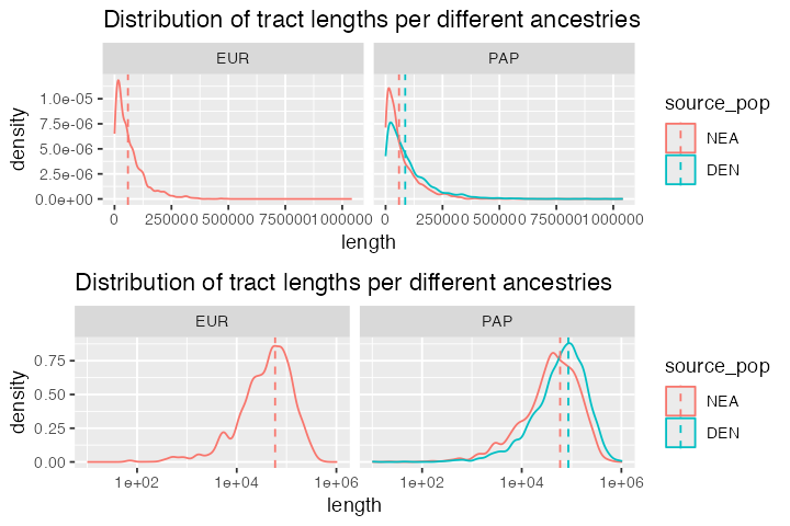
Pure msprime tree sequence
Finally, as a sanity check, let’s use the pure msprime
simulation example from the official
tspop documentation to test that ts_tracts()
behaves as expected even on a standard msprime tree-sequence
object.
First, let’s run the simulation code exactly as it is:
import msprime

pop_size = 500
sequence_length = 1e7
seed = 98765
rho = 3e-8

# Make the Demography object.
demography = msprime.Demography()
demography.add_population(name="RED", initial_size=pop_size)
#> Population(initial_size=500, growth_rate=0, name='RED', description='', extra_metadata={}, default_sampling_time=None, initially_active=None, id=0)
demography.add_population(name="BLUE", initial_size=pop_size)
#> Population(initial_size=500, growth_rate=0, name='BLUE', description='', extra_metadata={}, default_sampling_time=None, initially_active=None, id=1)
demography.add_population(name="ADMIX", initial_size=pop_size)
#> Population(initial_size=500, growth_rate=0, name='ADMIX', description='', extra_metadata={}, default_sampling_time=None, initially_active=None, id=2)
demography.add_population(name="ANC", initial_size=pop_size)
#> Population(initial_size=500, growth_rate=0, name='ANC', description='', extra_metadata={}, default_sampling_time=None, initially_active=None, id=3)
demography.add_admixture(
    time=100, derived="ADMIX", ancestral=["RED", "BLUE"], proportions=[0.5, 0.5]
)
#> Admixture(time=100, derived='ADMIX', ancestral=['RED', 'BLUE'], proportions=[0.5, 0.5])
demography.add_census(time=100.01) # Census is here!
#> CensusEvent(time=100.01)
demography.add_population_split(
    time=1000, derived=["RED", "BLUE"], ancestral="ANC"
)
#> PopulationSplit(time=1000, derived=['RED', 'BLUE'], ancestral='ANC')

# Simulate.
ts = msprime.sim_ancestry(
    samples={"RED": 0, "BLUE": 0, "ADMIX" : 2},
    demography=demography,
    random_seed=seed,
    sequence_length=sequence_length,
    recombination_rate=rho
)
Let’s save the msprime tree sequence to disk so that we can
load it into R (i.e., approximating what you might want to do should you
want to use ts_tracts() without running a slendr
simulation first):
Now let’s move to R again, load the tree sequence into
slendr and extract ancestry tracts from it using
ts_tracts():
sim_ts <- ts_load(reticulate::py$path)

squashed_tracts <- ts_tracts(sim_ts, census = 100.01, squashed = TRUE)
#>
#> PopAncestry summary
#> Number of ancestral populations:     2
#> Number of sample chromosomes:        4
#> Number of ancestors:             118
#> Total length of genomes:         40000000.000000
#> Ancestral coverage:          40000000.000000

head(squashed_tracts)
#> # A tibble: 6 × 4
#>   sample    left   right population
#>    <dbl>   <dbl>   <dbl>      <dbl>
#> 1      0       0  419848          0
#> 2      0  419848  483009          1
#> 3      0  483009 1475765          0
#> 4      0 1475765 2427904          1
#> 5      0 2427904 3635390          0
#> 6      0 3635390 4606954          1
tail(squashed_tracts)
#> # A tibble: 6 × 4
#>   sample    left    right population
#>    <dbl>   <dbl>    <dbl>      <dbl>
#> 1      3 7134130  7362300          1
#> 2      3 7362300  7369409          0
#> 3      3 7369409  7596783          1
#> 4      3 7596783  8289015          0
#> 5      3 8289015  8918727          1
#> 6      3 8918727 10000000          0
By setting squashed = FALSE, we get the full,
un-squashed ancestry segments, each with its appropriate ancestral node
ID:
full_tracts <- ts_tracts(sim_ts, census = 100.01, squashed = FALSE)
#>
#> PopAncestry summary
#> Number of ancestral populations:     2
#> Number of sample chromosomes:        4
#> Number of ancestors:             118
#> Total length of genomes:         40000000.000000
#> Ancestral coverage:          40000000.000000

head(full_tracts)
#> # A tibble: 6 × 5
#>   sample   left   right ancestor population
#>    <int>  <dbl>   <dbl>    <int>      <int>
#> 1      0      0   33027       74          0
#> 2      0  33027  155453       33          0
#> 3      0 155453  290542       46          0
#> 4      0 290542  419848       18          0
#> 5      0 419848  483009       83          1
#> 6      0 483009 1475765       28          0
tail(full_tracts)
#> # A tibble: 6 × 5
#>   sample    left    right ancestor population
#>    <int>   <dbl>    <dbl>    <int>      <int>
#> 1      3 8477625  8672850       94          1
#> 2      3 8672850  8849756       95          1
#> 3      3 8849756  8918727      131          1
#> 4      3 8918727  9165035       44          0
#> 5      3 9165035  9176562       47          0
#> 6      3 9176562 10000000       58          0
By comparing the two tables above to the pandas data frames in the tspop documentation, we can see that we obtained the same results.