Examples from the slendr paper

Note

Since the publication of the slendr paper, new versions of SLiM and slendr have been released. Specifically, the results in the paper are based on SLiM version 4.0.1 and slendr version 0.5. Whenever a new version of SLiM is released, there’s always a chance that some aspect of randomness in a simulation changes slightly, which affects the results even though the random seed is kept at the same value. As such, the figures in this paper (specifically the figure for Example 4 in our paper) will look slightly different. However, the results are still relevant and applicable, its just the presentation which has changed.

# workaround for GitHub actions getting "Killed" due to out of memory issues
# -- when running unit tests on GitHub, smaller amount of sequence will be
# simulated
if (Sys.getenv("RUNNER_OS") != "") {
  scaling <- 10 # use 10X less sequence on GitHub actions
} else {
  scaling <- 1 # but simulate normal amount of data otherwise
}

library(slendr)

library(dplyr)
#> 
#> Attaching package: 'dplyr'
#> The following objects are masked from 'package:stats':
#> 
#>     filter, lag
#> The following objects are masked from 'package:base':
#> 
#>     intersect, setdiff, setequal, union
library(ggplot2)
library(purrr)
library(tidyr)
library(cowplot)
library(forcats)

init_env()
#> The interface to all required Python modules has been activated.

SEED <- 42
set.seed(SEED)

# placeholder "figure" where a code chunk will be pasted
p_code <- ggplot() +
  geom_text(aes(x = 1, y = 1), label = "code will be here") +
  theme_void()

Example 1 (Figure 2)

Script from panel A

o <- population("o", time = 1, N = 100)
c <- population("c", time = 2500, N = 100, parent = o)
a <- population("a", time = 2800, N = 100, parent = c)
b <- population("b", time = 3700, N = 100, parent = a)
x1 <- population("x1", time = 4000, N = 15000, parent = c)
x2 <- population("x2", time = 4300, N = 15000, parent = x1)

gf <- gene_flow(from = b, to = x1, start = 5400, end = 5800, 0.1)

model <- compile_model(
  populations = list(o, a, b, c, x1, x2), gene_flow = gf,
  generation_time = 1, simulation_length = 6000
)

plot_model(model, sizes = FALSE, proportions = TRUE) # panel B

ts <- msprime(model, sequence_length = 100e6 / scaling, recombination_rate = 1e-8, random_seed = SEED) %>%
  ts_mutate(mutation_rate = 1e-8, random_seed = SEED)

samples <- ts_samples(ts) %>% group_by(pop) %>% sample_n(100)

# panel C
divergence <- ts_divergence(ts, split(samples$name, samples$pop))

# panel D
f4ratio <- ts_f4ratio(
  ts, X = filter(samples, pop %in% c("x1", "x2"))$name,
  A = "a_1", B = "b_1", C = "c_1", O = "o_1"
)

Complementary SLiM run from the same model

Plotting code

divergence <- divergence %>% mutate(pair = paste(x, "-", y))

f4ratio <- f4ratio %>% mutate(population = gsub("^(.*)_.*$", "\\1", X), alpha = alpha * 100)

p_ex1_divergence <- divergence %>%
  ggplot(aes(fct_reorder(pair, divergence), divergence)) +
  geom_point(size = 2.5) +
  xlab("population pair") + ylab("pairwise divergence") +
  theme_minimal() +
  theme(legend.position = "bottom",
        legend.text = element_text(size = 10),
        axis.text.x = element_text(hjust = 1, angle = 45, size = 8),
        axis.title.x = element_blank())

p_ex1_f4ratio <- f4ratio %>%
  ggplot(aes(population, alpha)) +
  geom_hline(yintercept = 0, linetype = 2) +
  geom_jitter(alpha = 0.5) +
  geom_boxplot(outlier.shape = NA, alpha = 0.7) +
  ylab(base::expression(italic("f")[4]~"-ratio ancestry proportion [%]")) +
  theme_minimal() +
  coord_cartesian(ylim = c(0, 20)) +
  theme(legend.position = "none",
        axis.text.x = element_text(size = 11),
        axis.title.x = element_blank(),
        panel.grid.major.x = element_blank())#; p_ex3_f4ratio

# let's avoid ggpubr as another dependency:
# https://github.com/kassambara/ggpubr/blob/master/R/as_ggplot.R#L27
p_ex1_legend <- ggdraw() + draw_grob(grid::grobTree(get_legend(p_ex1_divergence)))
#> Warning in get_plot_component(plot, "guide-box"): Multiple components found;
#> returning the first one. To return all, use `return_all = TRUE`.

p_ex1_model <- plot_model(model, sizes = FALSE, proportions = TRUE)

p_ex1 <- plot_grid(
  p_code,
  plot_grid(
    p_ex1_model,
    plot_grid(
      p_ex1_divergence + theme(legend.position = "none"),
      p_ex1_f4ratio,
      ncol = 2, rel_widths = c(1, 0.8), labels = c("C", "D")
    ),
    p_ex1_legend, nrow = 3, rel_heights = c(1, 1, 0.1),
    labels = "B"
  ),
  nrow = 1, labels = c("A", "")
)

p_ex1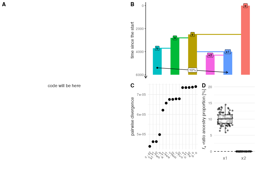

Example 2 (Figure 3)

Script from panel A

map <- world(xrange = c(0, 10), yrange = c(0, 10),
             landscape = region(center = c(5, 5), radius = 5))

p1 <- population("pop1", time = 1, N = 2000, map = map, competition = 0)
p2 <- population("pop2", time = 1, N = 2000, map = map, competition = 9)
p3 <- population("pop3", time = 1, N = 2000, map = map, competition = 6)
p4 <- population("pop4", time = 1, N = 2000, map = map, competition = 5)
p5 <- population("pop5", time = 1, N = 2000, map = map, competition = 4)
p6 <- population("pop6", time = 1, N = 2000, map = map, competition = 3)
p7 <- population("pop7", time = 1, N = 2000, map = map, competition = 2)
p8 <- population("pop8", time = 1, N = 2000, map = map, competition = 1)

model <- compile_model(
  populations = list(p1, p2, p3, p4, p5, p6, p7, p8),
  generation_time = 1, simulation_length = 5000, resolution = 0.1,
  mating = 0.1, dispersal = 0.05
)

ts <-
  slim(model, sequence_length = 10e6 / scaling, recombination_rate = 1e-8, random_seed = SEED) %>%
  ts_simplify() %>%
  ts_mutate(mutation_rate = 1e-7, random_seed = SEED)
#> Warning: Simplifying a non-recapitated tree sequence. Make sure this is what
#> you really want

locations <- ts_nodes(ts) %>% filter(time == max(time))

heterozygosity <- ts_samples(ts) %>%
  group_by(pop) %>%
  sample_n(100) %>%
  mutate(pi = ts_diversity(ts, name)$diversity)

Plotting code

p_ex2_clustering <- ggplot() +
  geom_sf(data = map) +
  geom_sf(data = locations, aes(color = pop), size = 0.05, alpha = 0.25) +
  facet_grid(. ~ pop, switch = "x") +
  xlab("spatial distributions emerged in the simulation") +
  theme(
    strip.background = element_blank(),
    strip.text = element_text(size = 11),
    panel.grid = element_blank(),
    axis.ticks = element_blank(),
    axis.text = element_blank(),
    panel.background = element_blank()
  ) +
  guides(color = "none")

p_ex2_diversity <- ggplot(heterozygosity, aes(pop, pi, color = pop)) +
  geom_violin(color = "black") +
  geom_jitter(alpha = 0.5) +
  labs(y = "individual heterozygosity") +
  guides(color = "none") +
  theme_minimal() +
  theme(axis.title.x = element_blank(),
        axis.text.x = element_blank(), panel.grid.major.x = element_blank(),
        plot.margin = margin(t = 0.2, r = 0.2, b = -0.1, l = 0.2, "cm"))

p_ex2 <- plot_grid(
  p_code,
  plot_grid(
    p_ex2_diversity,
    p_ex2_clustering +
      theme(plot.margin = margin(t = 0, r = 0.4, b = 0, l = 1.8, "cm")),
    nrow = 2,
    rel_heights = c(1, 0.5),
    labels = c("B", "C")
  ),
  nrow = 2, labels = c("A", ""), rel_heights = c(1.5, 1)
)

p_ex2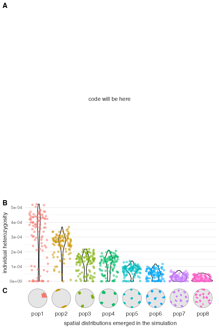

Example 3 (Figure 4)

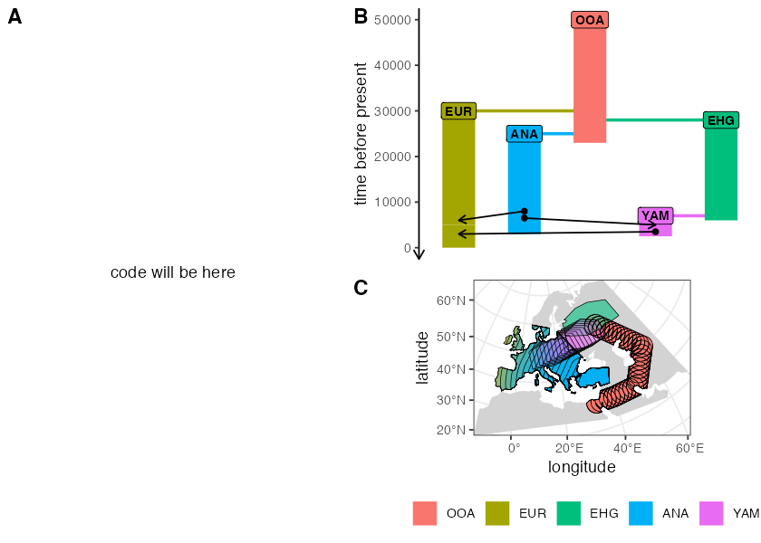
Script from panel A

map <- world(xrange = c(-13, 70), yrange = c(18, 65), crs = 3035)
#> Reading layer `ne_110m_land' from data source 
#>   `/private/var/folders/70/b_q2zdh116b9pfg29p03sx600000gn/T/RtmpEjQcFr/naturalearth/ne_110m_land.shp' 
#>   using driver `ESRI Shapefile'
#> Simple feature collection with 127 features and 3 fields
#> Geometry type: POLYGON
#> Dimension:     XY
#> Bounding box:  xmin: -180 ymin: -90 xmax: 180 ymax: 83.64513
#> Geodetic CRS:  WGS 84

R1 <- region(
  "EHG range", map,
  polygon = list(c(26, 55), c(38, 53), c(48, 53), c(60, 53),
                 c(60, 60), c(48, 63), c(38, 63), c(26, 60))
)
R2 <- region(
  "Europe", map,
  polygon = list(
    c(-8, 35), c(-5, 36), c(10, 38), c(20, 35), c(25, 35),
    c(33, 45), c(20, 58), c(-5, 60), c(-15, 50)
  )
)
R3 <- region(
  "Anatolia", map,
  polygon = list(c(28, 35), c(40, 35), c(42, 40),
                 c(30, 43), c(27, 40), c(25, 38))
)
R4 <- join(R2, R3)
R5 <- region(
  "YAM range", map,
  polygon = list(c(26, 50), c(38, 49), c(48, 50),
                 c(48, 56), c(38, 59), c(26, 56))
)

ooa_trajectory <- list(c(40, 30), c(50, 30), c(60, 40), c(45, 55))

map <- world(xrange = c(-13, 70), yrange = c(18, 65), crs = 3035)
#> Reading layer `ne_110m_land' from data source 
#>   `/private/var/folders/70/b_q2zdh116b9pfg29p03sx600000gn/T/RtmpEjQcFr/naturalearth/ne_110m_land.shp' 
#>   using driver `ESRI Shapefile'
#> Simple feature collection with 127 features and 3 fields
#> Geometry type: POLYGON
#> Dimension:     XY
#> Bounding box:  xmin: -180 ymin: -90 xmax: 180 ymax: 83.64513
#> Geodetic CRS:  WGS 84

ooa <- population(
  "OOA", time = 50000, N = 500, remove = 23000,
   map = map, center = c(33, 30), radius = 400e3
) %>%
  move(trajectory = ooa_trajectory, start = 50000, end = 40000, snapshots = 30)

ehg <- population(
  "EHG", time = 28000, N = 1000, parent = ooa, remove = 6000,
  map = map, polygon = R1
)

eur <- population(
  "EUR", time = 30000, N = 2000, parent = ooa,
  map = map, polygon = R2
) %>%
  resize(N = 10000, time = 5000, end = 0, how = "exponential")

ana <- population(
  "ANA", time = 25000, N = 4000, parent = ooa, remove = 3000,
  map = map, polygon = R3
) %>%
  expand_range(by = 3e6, start = 10000, end = 7000, polygon = R4, snapshots = 15)

yam <- population(
  "YAM", time = 7000, N = 600, parent = ehg, remove = 2500,
  map = map, polygon = R5
) %>%
  move(trajectory = list(c(15, 50)), start = 5000, end = 3000, snapshots = 10)

gf <- list(
  gene_flow(ana, to = yam, rate = 0.5, start = 6500, end = 5000),
  gene_flow(ana, to = eur, rate = 0.6, start = 8000, end = 6000),
  gene_flow(yam, to = eur, rate = 0.7, start = 3500, end = 3000)
)

model <- compile_model(
  populations = list(ooa, ehg, eur, ana, yam), gene_flow = gf,
  generation_time = 30, resolution = 10e3,
  competition = 150e3, mating = 120e3, dispersal = 90e3
)

samples <- schedule_sampling(
  model, times = seq(0, 50000, by = 1000),
  list(ehg, 20), list(ana, 20), list(yam, 20), list(eur, 20)
)

plot_model(model, sizes = FALSE)
plot_map(model)

ts <- slim(
  model, burnin = 200000, samples = samples, random_seed = SEED,
  sequence_length = 200000, recombination_rate = 1e-8
)

Plotting code

p_map <- plot_map(model) +
  theme(legend.position = "bottom") +
  guides(alpha = "none")

p_ex3 <- plot_grid(
  p_code,
  plot_grid(
    plot_model(model, sizes = FALSE),
    p_map,
    labels = c("B", "C"), nrow = 2, rel_heights = c(1, 1)
  ),
  ncol = 2, labels = c("A", ""), rel_widths = c(1, 1.2)
)

p_ex3

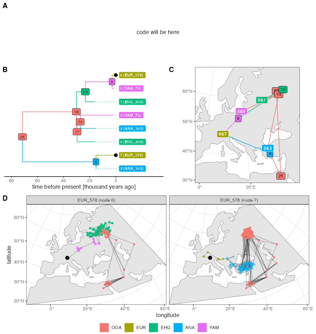
Example 4 (Figure 5)

Script from panel A

ts_small <- ts_simplify(ts, simplify_to = c("EUR_578", "YAM_75", "ANA_163", "EHG_208"))

# tskit uses zero-based indexing
tree <- ts_phylo(ts_small, i = 0 / scaling)
#> Starting checking the validity of tree...
#> Found number of tips: n = 8 
#> Found number of nodes: m = 7 
#> Done.
nodes <- ts_nodes(tree)
edges <- ts_edges(tree)

ancestors <- ts_ancestors(ts, "EUR_578")

Plotting code

library(ggtree)
#> ggtree v3.10.1 For help: https://yulab-smu.top/treedata-book/
#> 
#> If you use the ggtree package suite in published research, please cite
#> the appropriate paper(s):
#> 
#> Guangchuang Yu, David Smith, Huachen Zhu, Yi Guan, Tommy Tsan-Yuk Lam.
#> ggtree: an R package for visualization and annotation of phylogenetic
#> trees with their covariates and other associated data. Methods in
#> Ecology and Evolution. 2017, 8(1):28-36. doi:10.1111/2041-210X.12628
#> 
#> Guangchuang Yu.  Data Integration, Manipulation and Visualization of
#> Phylogenetic Trees (1st edition). Chapman and Hall/CRC. 2022,
#> doi:10.1201/9781003279242
#> 
#> Guangchuang Yu. Using ggtree to visualize data on tree-like structures.
#> Current Protocols in Bioinformatics. 2020, 69:e96. doi:10.1002/cpbi.96
#> 
#> 
#> Attaching package: 'ggtree'
#> The following object is masked from 'package:tidyr':
#> 
#>     expand

# prepare annotation table for ggtree linking R phylo node ID (not tskit integer
# ID!) of each node with its population name
df <- as_tibble(nodes) %>% select(node = phylo_id, pop)

abs_comma <- function (x, ...) {
  format(abs(x) / 1000, ..., scientific = FALSE, trim = TRUE)
}

highlight_nodes <- as_tibble(nodes) %>% dplyr::filter(name == "EUR_578") %>% .$phylo_id

p_tree <- ggtree(tree, aes(color = pop, fill = pop)) %<+% df +
  geom_tiplab(align = TRUE, geom = "label", offset = 2000,
              color = "white", fontface = "bold", size = 2.7) +
  geom_tiplab(align = TRUE, geom = NULL, linetype = "dotted", size = 0) +
  geom_point2(aes(subset = (node %in% highlight_nodes)), color = "black", size = 2.7) +
  geom_label2(aes(label = label, subset = !isTip),
              color = "black", size = 2.7) +
  theme_tree2() +
  theme(legend.position = "none") +
  xlab("time before present [thousand years ago]") +
  scale_x_continuous(limits = c(-80000, 31000), labels = abs_comma,
                     breaks = -c(100, 80, 60, 40, 20, 0) * 1000)
p_tree <- revts(p_tree)

# nodes$label <- ifelse(is.na(nodes$name), nodes$node_id, nodes$name)
nodes$label <- sapply(1:nrow(nodes), function(i) {
  if (is.na(nodes[i, ]$name))
    nodes[i, ]$node_id
  else {
    ind <- nodes[i, ]$name
    paste(nodes[!is.na(nodes$name) & nodes$name == ind, ]$node_id, collapse = "&")
  }
})

p_map <- ggplot() +
  geom_sf(data = map) +
  geom_sf(data = edges, aes(color = parent_pop), size = 0.5) +
  geom_sf_label(data = nodes[!nodes$sampled, ],
                aes(label = node_id, fill = pop), size = 3) +
  geom_sf_label(data = nodes[nodes$sampled, ],
                aes(label = label, fill = pop), size = 3,
                fontface = "bold", color = "white") +
  coord_sf(xlim = c(3177066.1, 7188656.9),
           ylim = c(757021.7, 5202983.3), expand = 0) +
  guides(fill = guide_legend("", override.aes = aes(label = ""))) +
  guides(color = "none") +
  scale_colour_discrete(drop = FALSE) +
  scale_fill_discrete(drop = FALSE) +
  theme_bw() +
  theme(legend.position = "bottom",
        axis.title.x = element_blank(),
        axis.title.y = element_blank())

chrom_names <- stats::setNames(
  c("EUR_578 (node 6)", "EUR_578 (node 7)"),
  unique(ancestors$node_id)
)

p_ancestors <- ggplot() +
  geom_sf(data = map) +
  geom_sf(data = ancestors, size = 0.5, alpha = 0.25) +
  geom_sf(data = sf::st_set_geometry(ancestors, "parent_location"),
          aes(shape = parent_pop, color = parent_pop)) +
  geom_sf(data = filter(ts_nodes(ts), name == "EUR_578"), size = 3) +
  coord_sf(expand = 0) +
  labs(x = "longitude", y = "latitude") +
  theme_bw() +
  facet_grid(. ~ node_id, labeller = labeller(node_id = chrom_names)) +
  theme(legend.position = "none")

p_legend <- ggdraw() + draw_grob(grid::grobTree(get_legend(p_map)))
#> Warning in get_plot_component(plot, "guide-box"): Multiple components found;
#> returning the first one. To return all, use `return_all = TRUE`.

p_ex4 <- plot_grid(
  p_code,
  plot_grid(p_tree + theme(legend.position = "none"),
            p_map + theme(legend.position = "none"),
            labels = c("B", "C"), rel_widths = c(1, 0.9)),
  p_ancestors,
  p_legend,
  labels = c("A", "", "D", ""),
  nrow = 4, rel_heights = c(0.5, 1, 1, 0.1)
)

p_ex4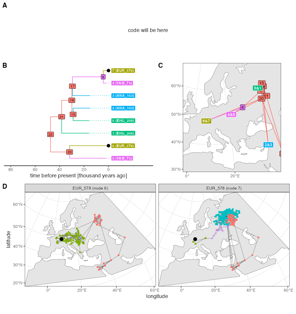

As explained on top of this page, the random number generation in the current SLiM is slightly different from the version 4.0.1 which was available at the time of writing of our paper. This is why the figure above looks a little different as well (different random generation implies different movement of individuals, and different individuals being sampled). For the record, here’s the original figure used in our paper which was also originally part of this vignette:

Run time of each code example from the paper

The following times were measured on a 16’’ MacBook Pro with the Apple M1 Pro chip (2021 model), 32 GB RAM, running macOS Ventura Version 13.1.

example	time	units
ex1	6.0739652	mins
ex2	12.4129678	mins
ex3	2.1079260	mins
ex4	0.4259529	secs

In the table above, ex1, ex2, ex3, and ex4 correspond to runtimes of code shown in one of the four example figures in the slendr paper.