Compile a slendr demographic model — compile

First, compiles the vectorized population spatial maps into a series of binary raster PNG files, which is the format that SLiM understands and uses it to define population boundaries. Then extracts the demographic model defined by the user (i.e. population divergences and gene flow events) into a series of tables which are later used by the built-in SLiM script to program the timing of simulation events.

Usage

compile_model(
  populations,
  generation_time,
  path = NULL,
  resolution = NULL,
  competition = NULL,
  mating = NULL,
  dispersal = NULL,
  gene_flow = list(),
  overwrite = FALSE,
  force = FALSE,
  simulation_length = NULL,
  direction = NULL,
  serialize = TRUE,
  slim_script = NULL,
  description = "",
  sim_length = NULL
)

Arguments

populations: Object(s) of the slendr_pop class (multiple objects need to be specified in a list)
generation_time: Generation time (in model time units)
path: Output directory for the model configuration files which will be loaded by the backend SLiM script. If NULL, model configuration files will be saved to a temporary directory.
resolution: How many distance units per pixel?
competition, mating: Maximum spatial competition and mating choice distance
dispersal: Standard deviation of the normal distribution of the parent-offspring distance
gene_flow: Gene flow events generated by the gene_flow function (either a list of data.frame objects in the format defined by the gene_flow function, or a single data.frame)
overwrite: Completely delete the specified directory, in case it already exists, and create a new one?
force: Force a deletion of the model directory if it is already present? Useful for non-interactive uses. In an interactive mode, the user is asked to confirm the deletion manually.
simulation_length: Total length of the simulation (required for forward time models, optional for models specified in backward time units which by default run to "the present time")
direction: Intended direction of time. Under normal circumstances this parameter is inferred from the model and does not need to be set manually.
serialize: Should model files be serialized to disk? If not, only an R model object will be returned but no files will be created. This speeds up simulation with msprime but prevents using the SLiM back end.
slim_script: Path to a SLiM script to be used for executing the model (by default, a bundled backend script will be used). If NULL, the SLiM script bundled with slendr will be used.
description: Optional short description of the model
sim_length: Deprecated. Use simulation_length instead.

Value

Compiled slendr_model model object which encapsulates all information about the specified model (which populations are involved, when and how much gene flow should occur, what is the spatial resolution of a map, and what spatial dispersal and mating parameters should be used in a SLiM simulation, if applicable)

Examples

# spatial definitions -----------------------------------------------------

# create a blank abstract world 1000x1000 distance units in size
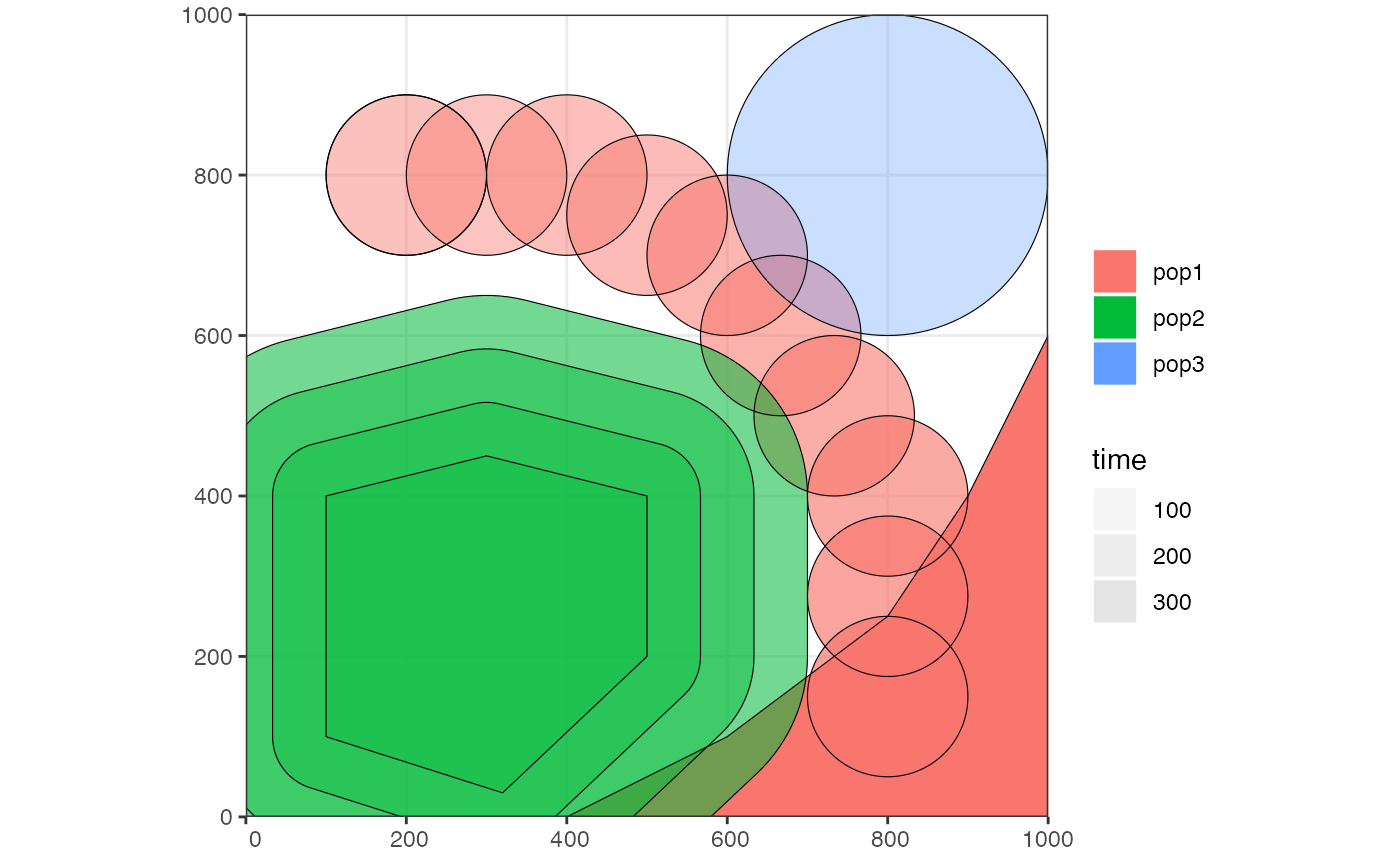
map <- world(xrange = c(0, 1000), yrange = c(0, 1000), landscape = "blank")

# create a circular population with the center of a population boundary at
# [200, 800] and a radius of 100 distance units, 1000 individuals at time 1
# occupying a map just specified
pop1 <- population("pop1", N = 1000, time = 1,
                   map = map, center = c(200, 800), radius = 100)

# printing a population object to a console shows a brief summary
pop1
#> slendr 'population' object 
#> -------------------------- 
#> name: pop1 
#> habitat: terrestrial
#> 
#> number of spatial maps: 1 
#> map: abstract spatial landscape with custom features
#> stays until the end of the simulation
#> 
#> population history overview:
#>   - time 1: created as an ancestral population (N = 1000)

# create another population occupying a polygon range, splitting from pop1
# at a given time point (note that specifying a map is not necessary because
# it is "inherited" from the parent)
pop2 <- population("pop2", N = 100, time = 50, parent = pop1,
                        polygon = list(c(100, 100), c(320, 30), c(500, 200),
                                  c(500, 400), c(300, 450), c(100, 400)))

pop3 <- population("pop3", N = 200, time = 80, parent = pop2,
                   center = c(800, 800), radius = 200)

# move "pop1" to another location along a specified trajectory and saved the
# resulting object to the same variable (the number of intermediate spatial
# snapshots can be also determined automatically by leaving out the
# `snapshots = ` argument)
pop1_moved <- move(pop1, start = 100, end = 200, snapshots = 6,
                   trajectory = list(c(600, 820), c(800, 400), c(800, 150)))
pop1_moved
#> slendr 'population' object 
#> -------------------------- 
#> name: pop1 
#> habitat: terrestrial
#> 
#> number of spatial maps: 10 
#> map: abstract spatial landscape with custom features
#> stays until the end of the simulation
#> 
#> population history overview:
#>   - time 1: created as an ancestral population (N = 1000)
#>   - time 100-200: movement across a landscape

# many slendr functions are pipe-friendly, making it possible to construct
# pipelines which construct entire history of a population
pop1 <- population("pop1", N = 1000, time = 1,
                   map = map, center = c(200, 800), radius = 100) %>%
  move(start = 100, end = 200, snapshots = 6,
       trajectory = list(c(400, 800), c(600, 700), c(800, 400), c(800, 150))) %>%
  set_range(time = 300, polygon = list(
    c(400, 0), c(1000, 0), c(1000, 600), c(900, 400), c(800, 250),
    c(600, 100), c(500, 50))
  )

# population ranges can expand by a given distance in all directions
pop2 <- expand_range(pop2, by = 200, start = 50, end = 150, snapshots = 3)

# we can check the positions of all populations interactively by plotting their
# ranges together on a single map
plot_map(pop1, pop2, pop3)


# gene flow events --------------------------------------------------------

# individual gene flow events can be saved to a list
gf <- list(
  gene_flow(from = pop1, to = pop3, start = 150, end = 200, rate = 0.15),
  gene_flow(from = pop1, to = pop2, start = 300, end = 330, rate = 0.25)
)

# compilation -------------------------------------------------------------

# compile model components in a serialized form to dist, returning a single
# slendr model object (in practice, the resolution should be smaller)
model <- compile_model(
  populations = list(pop1, pop2, pop3), generation_time = 1,
  resolution = 100, simulation_length = 500,
  competition = 5, mating = 5, dispersal = 1
)