Update the population range — set

This function allows a more manual control of spatial map changes in addition to the expand and move functions

Usage

set_range(
  pop,
  time,
  center = NULL,
  radius = NULL,
  polygon = NULL,
  lock = FALSE
)

Arguments

pop: Object of the class slendr_pop
time: Time of the change
center: Two-dimensional vector specifying the center of the circular range
radius: Radius of the circular range
polygon: List of vector pairs, defining corners of the polygon range (see also the region argument) or a geographic region of the class slendr_region from which the polygon coordinates will be extracted
lock: Maintain the same density of individuals. If FALSE (the default), the number of individuals in the population will not change. If TRUE, the number of individuals simulated will be changed (increased or decreased) appropriately, to match the new population range area.

Value

Object of the class slendr_pop, which contains population parameters such as name, time of appearance in the simulation, parent population (if any), and its spatial parameters such as map and spatial boundary.

Examples

# spatial definitions -----------------------------------------------------

# create a blank abstract world 1000x1000 distance units in size
map <- world(xrange = c(0, 1000), yrange = c(0, 1000), landscape = "blank")

# create a circular population with the center of a population boundary at
# [200, 800] and a radius of 100 distance units, 1000 individuals at time 1
# occupying a map just specified
pop1 <- population("pop1", N = 1000, time = 1,
                   map = map, center = c(200, 800), radius = 100)

# printing a population object to a console shows a brief summary
pop1
#> slendr 'population' object 
#> -------------------------- 
#> name: pop1 
#> habitat: terrestrial
#> 
#> number of spatial maps: 1 
#> map: abstract spatial landscape with custom features
#> stays until the end of the simulation
#> 
#> population history overview:
#>   - time 1: created as an ancestral population (N = 1000)

# create another population occupying a polygon range, splitting from pop1
# at a given time point (note that specifying a map is not necessary because
# it is "inherited" from the parent)
pop2 <- population("pop2", N = 100, time = 50, parent = pop1,
                        polygon = list(c(100, 100), c(320, 30), c(500, 200),
                                  c(500, 400), c(300, 450), c(100, 400)))

pop3 <- population("pop3", N = 200, time = 80, parent = pop2,
                   center = c(800, 800), radius = 200)

# move "pop1" to another location along a specified trajectory and saved the
# resulting object to the same variable (the number of intermediate spatial
# snapshots can be also determined automatically by leaving out the
# `snapshots = ` argument)
pop1_moved <- move(pop1, start = 100, end = 200, snapshots = 6,
                   trajectory = list(c(600, 820), c(800, 400), c(800, 150)))
pop1_moved
#> slendr 'population' object 
#> -------------------------- 
#> name: pop1 
#> habitat: terrestrial
#> 
#> number of spatial maps: 10 
#> map: abstract spatial landscape with custom features
#> stays until the end of the simulation
#> 
#> population history overview:
#>   - time 1: created as an ancestral population (N = 1000)
#>   - time 100-200: movement across a landscape

# many slendr functions are pipe-friendly, making it possible to construct
# pipelines which construct entire history of a population
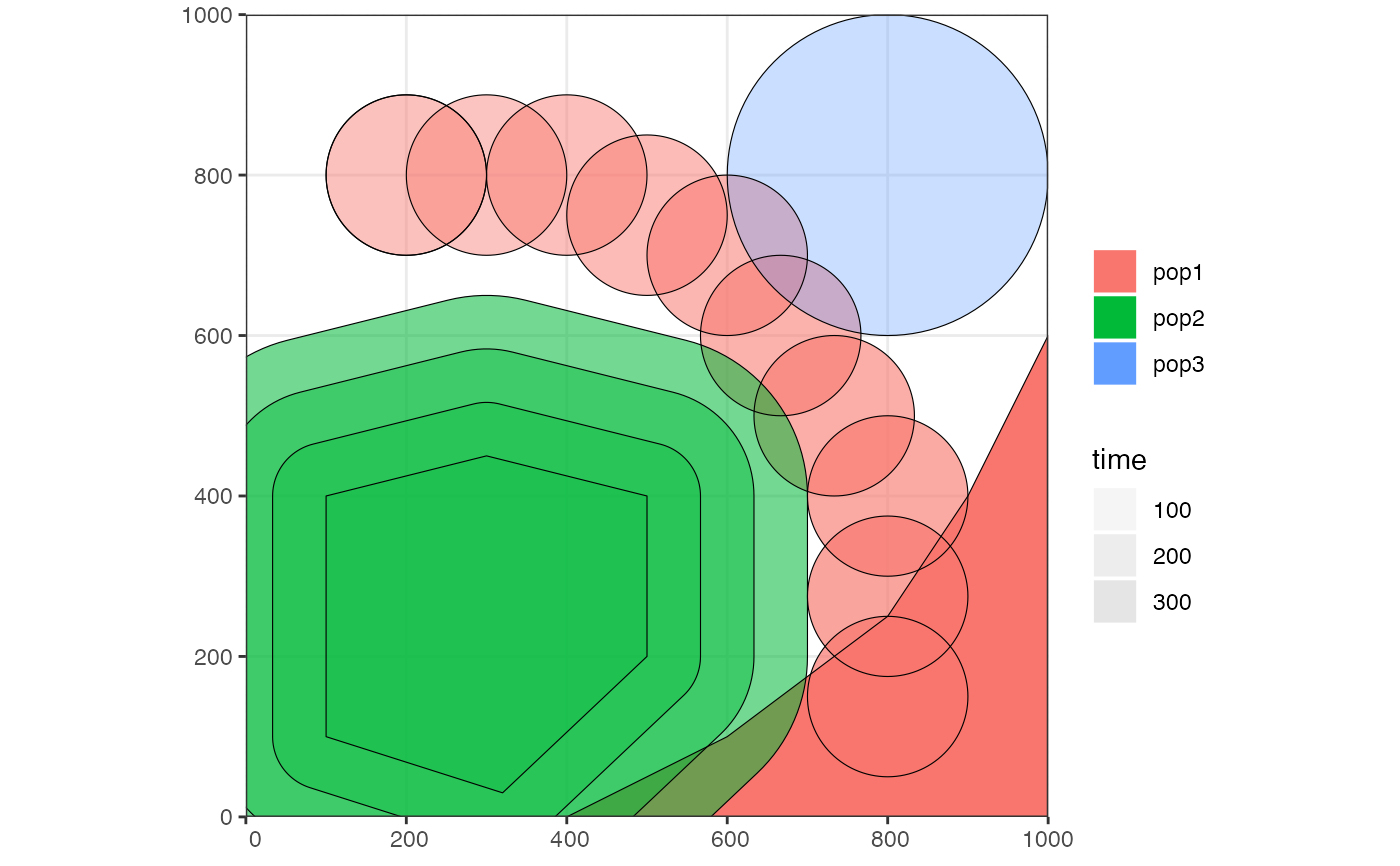
pop1 <- population("pop1", N = 1000, time = 1,
                   map = map, center = c(200, 800), radius = 100) %>%
  move(start = 100, end = 200, snapshots = 6,
       trajectory = list(c(400, 800), c(600, 700), c(800, 400), c(800, 150))) %>%
  set_range(time = 300, polygon = list(
    c(400, 0), c(1000, 0), c(1000, 600), c(900, 400), c(800, 250),
    c(600, 100), c(500, 50))
  )

# population ranges can expand by a given distance in all directions
pop2 <- expand_range(pop2, by = 200, start = 50, end = 150, snapshots = 3)

# we can check the positions of all populations interactively by plotting their
# ranges together on a single map
plot_map(pop1, pop2, pop3)


# gene flow events --------------------------------------------------------

# individual gene flow events can be saved to a list
gf <- list(
  gene_flow(from = pop1, to = pop3, start = 150, end = 200, rate = 0.15),
  gene_flow(from = pop1, to = pop2, start = 300, end = 330, rate = 0.25)
)

# compilation -------------------------------------------------------------

# compile model components in a serialized form to dist, returning a single
# slendr model object (in practice, the resolution should be smaller)
model <- compile_model(
  populations = list(pop1, pop2, pop3), generation_time = 1,
  resolution = 100, simulation_length = 500,
  competition = 5, mating = 5, dispersal = 1
)