Traditional, non-spatial models • slendr

The biggest selling point of the slendr package is that you can program spatiotemporal population genetics models in R and have them execute automatically in SLiM. However, there are several reasons why you might be interested in using slendr even for non-spatial models. First, R is a language that many scientists already know, and being able to simulate data from the comfort of an R interface significantly lowers the barrier of entry. Second, because slendr makes SLiM appear almost as if it were just another R library, running simulations (spatial and non-spatial), fitting models, exploring parameter grids, calculating statistics, and visualization of results can be all be performed without leaving the R interface.

In this vignette, we will demonstrate how to program non-spatial models in slendr. However, we should start by noting that there is almost no difference between code for non-spatial and spatial models in slendr. The only visible difference is that spatial models include a map = argument in the population() constructor function of ancestral population(s), and non-spatial models do not. That’s it, that’s the difference. Switching between spatial and non-spatial models is performed internally by the package, without any user intervention.

To make the comparison clearer, we will use the example from the slendr landing page, but we will implement it in a non-spatial context (i.e., as a traditional random mating simulation).

First, let’s define population objects, splits, and other demographic events (note the missing map argument, which is set to FALSE by default):

library(slendr)

init_env()

#> The interface to all required Python modules has been activated.

# African ancestral population
afr <- population("AFR", time = 100000, N = 3000)

# first migrants out of Africa
ooa <- population("OOA", parent = afr, time = 60000, N = 500, remove = 23000) %>%
  resize(N = 2000, time = 40000, how = "step")

# Eastern hunter-gatherers
ehg <- population("EHG", parent = ooa, time = 28000, N = 1000, remove = 6000)

# European population
eur <- population("EUR", parent = ehg, time = 25000, N = 2000) %>%
  resize(N = 10000, how = "exponential", time = 5000, end = 0)

# Anatolian farmers
ana <- population("ANA", time = 28000, N = 3000, parent = ooa, remove = 4000)

# Yamnaya steppe population
yam <- population("YAM", time = 7000, N = 500, parent = ehg, remove = 2500)

We can define gene flow events in the same way as we did for the spatial model:

gf <- list(
  gene_flow(from = ana, to = yam, rate = 0.5, start = 6500, end = 6400),
  gene_flow(from = ana, to = eur, rate = 0.5, start = 8000, end = 6000),
  gene_flow(from = yam, to = eur, rate = 0.75, start = 4000, end = 3000)
)

The compilation step is also the same. The only (internal) difference is that we skip the rasterization of vector maps that is performed for spatial models in order to control and restrict population boundaries:

model <- compile_model(
  populations = list(afr, ooa, ehg, eur, ana, yam),
  gene_flow = gf, generation_time = 30,
  time_units = "years before present"
)

Using the plot_map() function doesn’t make sense, as there are no spatial maps to plot. However, we can still plot the demographic graph, verifying that the model has been specified correctly using the function plot_model() as shown below.

Let’s say we also want to schedule specific sampling events at specific times (which record only specified individuals in a tree sequence). We can use schedule_sampling() to do just that:

samples <- schedule_sampling(
  model,
  times = c(0, 5000, 12000, 20000, 35000, 39000, 43000),
  list(eur, 3), list(ehg, 1), list(yam, 1), list(ana, 3), list(ooa, 1), list(afr, 1)
)

Because it’s not just the model itself that’s useful to visually verify (which is the main purpose of plot_model()) but also the sampling scheme, slendr makes it possible to overlay the numbers of individuals scheduled for tree-sequence recording from each lineage at each timepoint:

plot_model(model, samples = samples)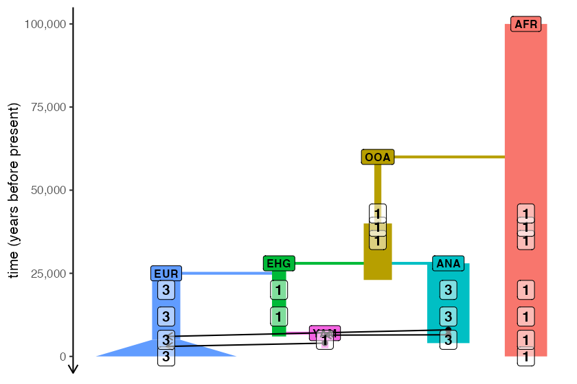

Even the final step—execution of the model in SLiM—is the same, using the built-in slim() function:

ts_slim <- slim(model, sequence_length = 100000, recombination_rate = 0)

Even for non-spatial models, this function still uses the same SLiM back end script used for spatial models. The only difference is that all spatial features are switched off, making the model run as a simple random-mating simulation.

Given that we are running a non-spatial simulation, you might wonder if it wouldn’t be more efficient to use a coalescent simulator. Indeed, slendr also provides an alternative msprime back end just for this purpose. We could run the exact same simulation with msprime like this:

ts_msprime <- msprime(model, sequence_length = 100000, recombination_rate = 0)

In fact, because both SLiM and msprime back ends save outputs in a tree sequence format, we can analyse them using the same tools. See this vignette for more information about tree sequence analysis with slendr, and for more discussion on alternative simulation back ends and more extensive examples of data analysis with tree sequences you can read this tutorial.

Extracting parameters from a model or tree sequences

In some situations (such as when model parameters are drawn from random distributions and we need to know which parameters had been used after the simulations), function extract_parameters() can be used. This function peeks into a slendr tree sequence object and extract parameters of the original slendr model:

extract_parameters(ts_msprime)

#> $splits
#>   pop parent    N   time remove
#> 1 AFR   <NA> 3000 100000     NA
#> 2 OOA    AFR  500  60000  23000
#> 3 EHG    OOA 1000  28000   6000
#> 5 ANA    OOA 3000  28000   4000
#> 4 EUR    EHG 2000  25000     NA
#> 6 YAM    EHG  500   7000   2500
#> 
#> $gene_flows
#>   from  to start  end rate
#> 1  ANA YAM  6500 6400 0.50
#> 2  ANA EUR  8000 6000 0.50
#> 3  YAM EUR  4000 3000 0.75
#> 
#> $resizes
#>   pop         how     N  time end
#> 1 OOA        step  2000 40000  NA
#> 2 EUR exponential 10000  5000   0

For completeness, although this isn’t relevant in this example either, the function can also get parameters from any compiled model. For instance, we can check which parameters were used to compile the built-in slendr introgression model by running:

introgression_model <- read_model(path = system.file("extdata/models/introgression", package = "slendr"))

extract_parameters(introgression_model)

#> $splits
#>   pop parent    N    time remove
#> 1  CH   <NA>   10 6500000     NA
#> 2 AFR     CH   10 6000000     NA
#> 3 NEA    AFR   10  600000  40000
#> 4 EUR    AFR 5000   70000     NA
#> 
#> $gene_flows
#>   from  to start   end rate
#> 1  NEA EUR 55000 45000 0.03

As we can see, extract_parameters() returns a list of data frames, one data frame for each aspect of a demographic model (where applicable).