Define a population — population • slendr

Defines the parameters of a population (non-spatial and spatial).

Usage

population(
  name,
  time,
  N,
  parent = NULL,
  map = FALSE,
  center = NULL,
  radius = NULL,
  polygon = NULL,
  remove = NULL,
  intersect = TRUE,
  competition = NA,
  mating = NA,
  dispersal = NA,
  dispersal_fun = NULL,
  aquatic = FALSE
)

Arguments

name: Name of the population
time: Time of the population's first appearance
N: Number of individuals at the time of first appearance
parent: Parent population object or NULL (which indicates that the population does not have an ancestor, as it is the first population in its "lineage")
map: Object of the type slendr_map which defines the world context (created using the world function). If the value FALSE is provided, a non-spatial model will be run.
center: Two-dimensional vector specifying the center of the circular range
radius: Radius of the circular range
polygon: List of vector pairs, defining corners of the polygon range or a geographic region of the class slendr_region from which the polygon coordinates will be extracted (see the region() function)
remove: Time at which the population should be removed
intersect: Intersect the population's boundaries with landscape features?
competition, mating: Maximum spatial competition and mating choice distance
dispersal: Standard deviation of the normal distribution of the distance that offspring disperses from its parent
dispersal_fun: Distribution function governing the dispersal of offspring. One of "normal", "uniform", "cauchy", "exponential", or "brownian" (in which vertical and horizontal displacements are drawn from a normal distribution independently).
aquatic: Is the species aquatic (FALSE by default, i.e. terrestrial species)?

Value

Object of the class slendr_pop, which contains population parameters such as name, time of appearance in the simulation, parent population (if any), and its spatial parameters such as map and spatial boundary.

Details

There are four ways to specify a spatial boundary: i) circular range specified using a center coordinate and a radius, ii) polygon specified as a list of two-dimensional vector coordinates, iii) polygon as in ii), but defined (and named) using the region function, iv) with just a world map specified (circular or polygon range parameters set to the default NULL value), the population will be allowed to occupy the entire landscape.

Note that because slendr models have to accomodate both SLiM and msprime back ends, population sizes and split times are rounded to the nearest integer value.

Examples

# spatial definitions -----------------------------------------------------

# create a blank abstract world 1000x1000 distance units in size
map <- world(xrange = c(0, 1000), yrange = c(0, 1000), landscape = "blank")

# create a circular population with the center of a population boundary at
# [200, 800] and a radius of 100 distance units, 1000 individuals at time 1
# occupying a map just specified
pop1 <- population("pop1", N = 1000, time = 1,
                   map = map, center = c(200, 800), radius = 100)

# printing a population object to a console shows a brief summary
pop1
#> slendr 'population' object 
#> -------------------------- 
#> name: pop1 
#> habitat: terrestrial
#> 
#> number of spatial maps: 1 
#> map: abstract spatial landscape with custom features
#> stays until the end of the simulation
#> 
#> population history overview:
#>   - time 1: created as an ancestral population (N = 1000)

# create another population occupying a polygon range, splitting from pop1
# at a given time point (note that specifying a map is not necessary because
# it is "inherited" from the parent)
pop2 <- population("pop2", N = 100, time = 50, parent = pop1,
                        polygon = list(c(100, 100), c(320, 30), c(500, 200),
                                  c(500, 400), c(300, 450), c(100, 400)))

pop3 <- population("pop3", N = 200, time = 80, parent = pop2,
                   center = c(800, 800), radius = 200)

# move "pop1" to another location along a specified trajectory and saved the
# resulting object to the same variable (the number of intermediate spatial
# snapshots can be also determined automatically by leaving out the
# `snapshots = ` argument)
pop1_moved <- move(pop1, start = 100, end = 200, snapshots = 6,
                   trajectory = list(c(600, 820), c(800, 400), c(800, 150)))
pop1_moved
#> slendr 'population' object 
#> -------------------------- 
#> name: pop1 
#> habitat: terrestrial
#> 
#> number of spatial maps: 10 
#> map: abstract spatial landscape with custom features
#> stays until the end of the simulation
#> 
#> population history overview:
#>   - time 1: created as an ancestral population (N = 1000)
#>   - time 100-200: movement across a landscape

# many slendr functions are pipe-friendly, making it possible to construct
# pipelines which construct entire history of a population
pop1 <- population("pop1", N = 1000, time = 1,
                   map = map, center = c(200, 800), radius = 100) %>%
  move(start = 100, end = 200, snapshots = 6,
       trajectory = list(c(400, 800), c(600, 700), c(800, 400), c(800, 150))) %>%
  set_range(time = 300, polygon = list(
    c(400, 0), c(1000, 0), c(1000, 600), c(900, 400), c(800, 250),
    c(600, 100), c(500, 50))
  )

# population ranges can expand by a given distance in all directions
pop2 <- expand_range(pop2, by = 200, start = 50, end = 150, snapshots = 3)

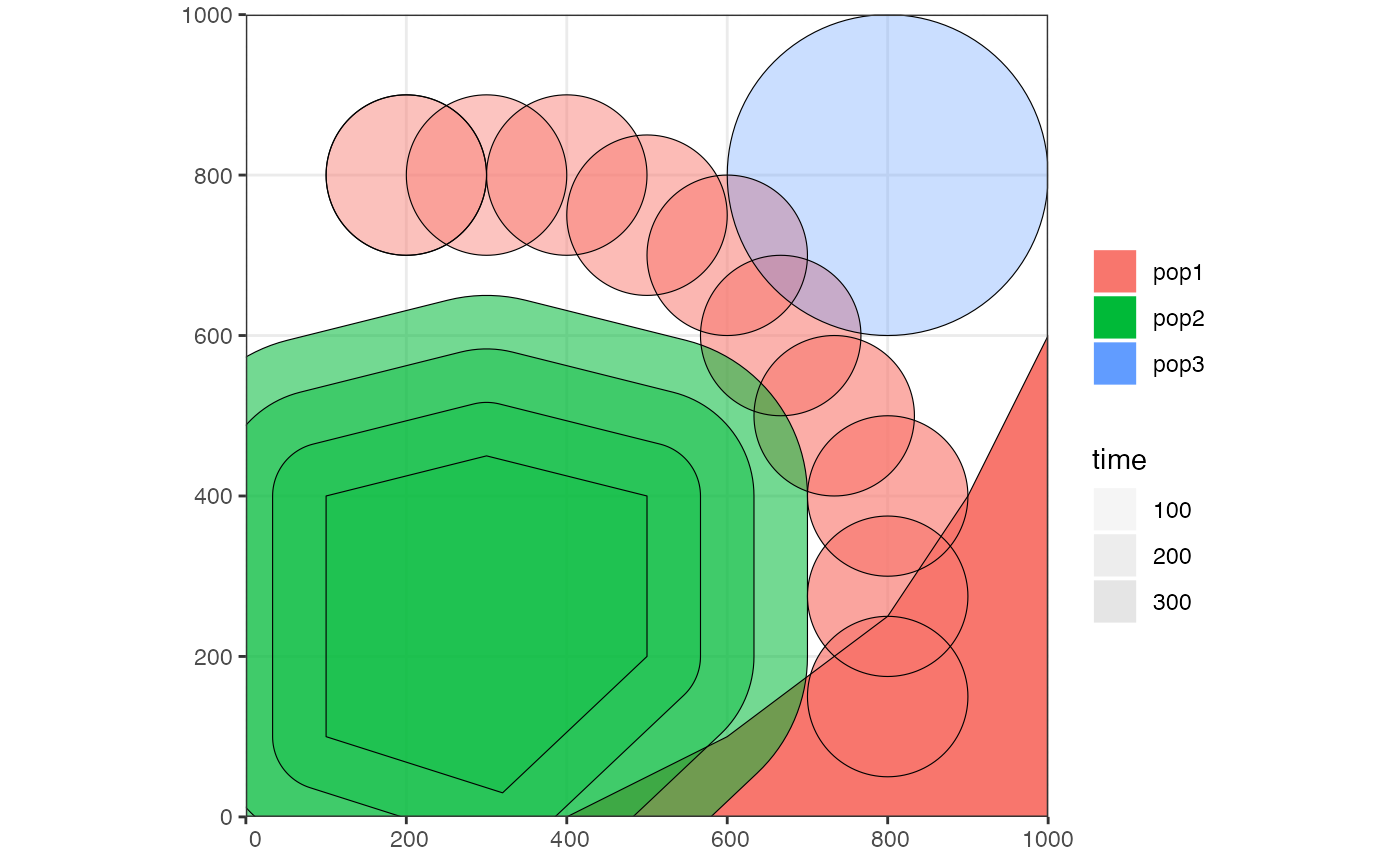
# we can check the positions of all populations interactively by plotting their
# ranges together on a single map
plot_map(pop1, pop2, pop3)


# gene flow events --------------------------------------------------------

# individual gene flow events can be saved to a list
gf <- list(
  gene_flow(from = pop1, to = pop3, start = 150, end = 200, rate = 0.15),
  gene_flow(from = pop1, to = pop2, start = 300, end = 330, rate = 0.25)
)

# compilation -------------------------------------------------------------

# compile model components in a serialized form to dist, returning a single
# slendr model object (in practice, the resolution should be smaller)
model <- compile_model(
  populations = list(pop1, pop2, pop3), generation_time = 1,
  resolution = 100, simulation_length = 500,
  competition = 5, mating = 5, dispersal = 1
)