Move the population to a new location in a given amount of time

This function defines a displacement of a population along a given trajectory in a given time frame

Usage

move(
  pop,
  trajectory,
  end,
  start,
  overlap = 0.8,
  snapshots = NULL,
  verbose = TRUE
)

Arguments

pop: Object of the class slendr_pop
trajectory: List of two-dimensional vectors (longitude, latitude) specifying the migration trajectory
start, end: Start/end points of the population migration
overlap: Minimum overlap between subsequent spatial boundaries
snapshots: The number of intermediate snapshots (overrides the overlap parameter)
verbose: Show the progress of searching through the number of sufficient snapshots?

Value

Object of the class slendr_pop, which contains population parameters such as name, time of appearance in the simulation, parent population (if any), and its spatial parameters such as map and spatial boundary.

Examples

# spatial definitions -----------------------------------------------------

# create a blank abstract world 1000x1000 distance units in size
map <- world(xrange = c(0, 1000), yrange = c(0, 1000), landscape = "blank")

# create a circular population with the center of a population boundary at
# [200, 800] and a radius of 100 distance units, 1000 individuals at time 1
# occupying a map just specified
pop1 <- population("pop1", N = 1000, time = 1,
                   map = map, center = c(200, 800), radius = 100)

# printing a population object to a console shows a brief summary
pop1
#> slendr 'population' object 
#> -------------------------- 
#> name: pop1 
#> habitat: terrestrial
#> 
#> number of spatial maps: 1 
#> map: abstract spatial landscape with custom features
#> stays until the end of the simulation
#> 
#> population history overview:
#>   - time 1: created as an ancestral population (N = 1000)

# create another population occupying a polygon range, splitting from pop1
# at a given time point (note that specifying a map is not necessary because
# it is "inherited" from the parent)
pop2 <- population("pop2", N = 100, time = 50, parent = pop1,
                        polygon = list(c(100, 100), c(320, 30), c(500, 200),
                                  c(500, 400), c(300, 450), c(100, 400)))

pop3 <- population("pop3", N = 200, time = 80, parent = pop2,
                   center = c(800, 800), radius = 200)

# move "pop1" to another location along a specified trajectory and saved the
# resulting object to the same variable (the number of intermediate spatial
# snapshots can be also determined automatically by leaving out the
# `snapshots = ` argument)
pop1_moved <- move(pop1, start = 100, end = 200, snapshots = 6,
                   trajectory = list(c(600, 820), c(800, 400), c(800, 150)))
pop1_moved
#> slendr 'population' object 
#> -------------------------- 
#> name: pop1 
#> habitat: terrestrial
#> 
#> number of spatial maps: 10 
#> map: abstract spatial landscape with custom features
#> stays until the end of the simulation
#> 
#> population history overview:
#>   - time 1: created as an ancestral population (N = 1000)
#>   - time 100-200: movement across a landscape

# many slendr functions are pipe-friendly, making it possible to construct
# pipelines which construct entire history of a population
pop1 <- population("pop1", N = 1000, time = 1,
                   map = map, center = c(200, 800), radius = 100) %>%
  move(start = 100, end = 200, snapshots = 6,
       trajectory = list(c(400, 800), c(600, 700), c(800, 400), c(800, 150))) %>%
  set_range(time = 300, polygon = list(
    c(400, 0), c(1000, 0), c(1000, 600), c(900, 400), c(800, 250),
    c(600, 100), c(500, 50))
  )

# population ranges can expand by a given distance in all directions
pop2 <- expand_range(pop2, by = 200, start = 50, end = 150, snapshots = 3)

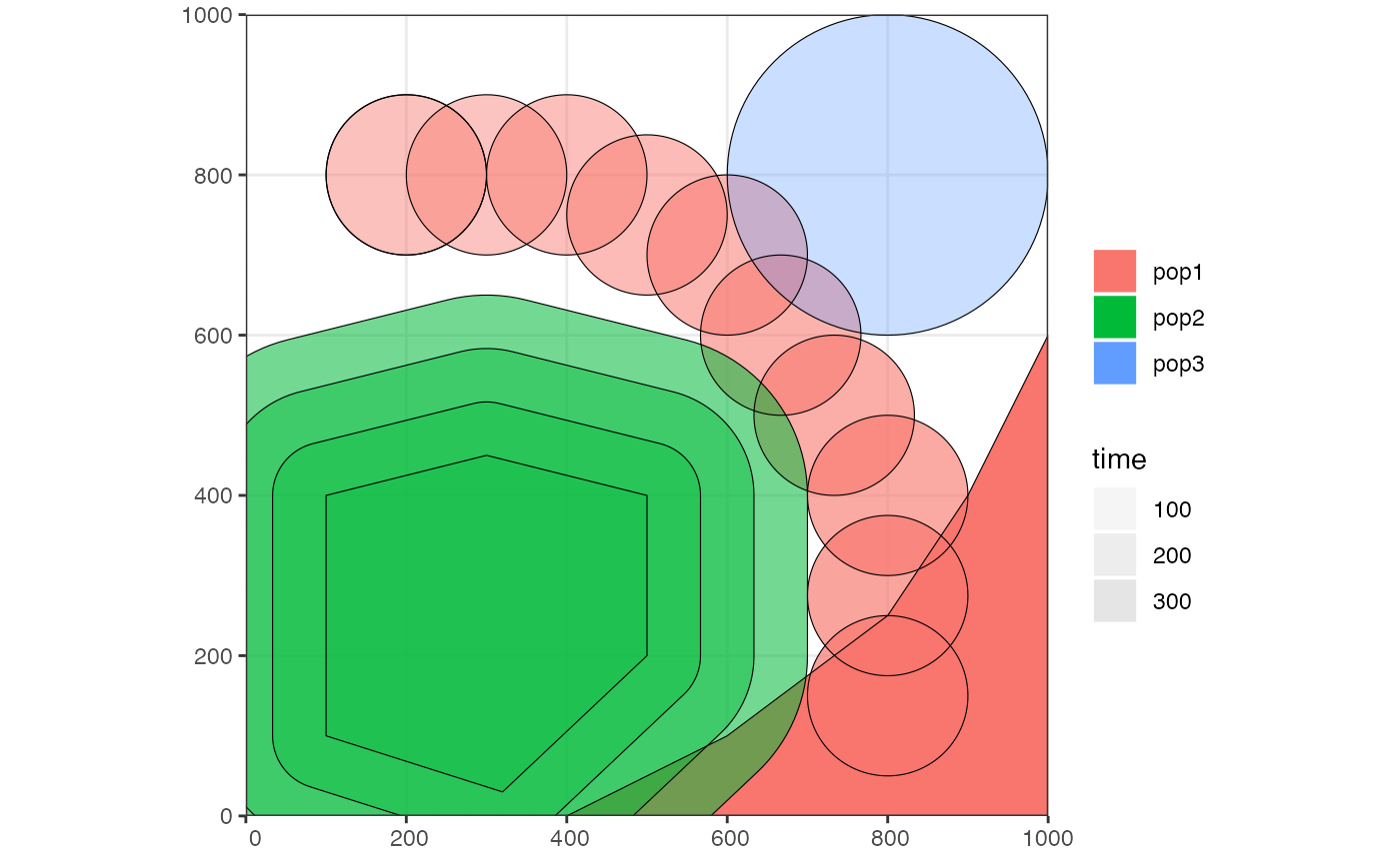
# we can check the positions of all populations interactively by plotting their
# ranges together on a single map
plot_map(pop1, pop2, pop3)


# gene flow events --------------------------------------------------------

# individual gene flow events can be saved to a list
gf <- list(
  gene_flow(from = pop1, to = pop3, start = 150, end = 200, rate = 0.15),
  gene_flow(from = pop1, to = pop2, start = 300, end = 330, rate = 0.25)
)

# compilation -------------------------------------------------------------

# compile model components in a serialized form to dist, returning a single
# slendr model object (in practice, the resolution should be smaller)
model <- compile_model(
  populations = list(pop1, pop2, pop3), generation_time = 1,
  resolution = 100, simulation_length = 500,
  competition = 5, mating = 5, dispersal = 1
)